深度学习

Machine Learning - Android Ng

3.1. 神经网络概论

尝试模仿（mimic）人脑
用处
- speech -> images -> text(NLP) -> …
每个神经元接受一些输入，做一些计算，然后将输出送给下一个神经元

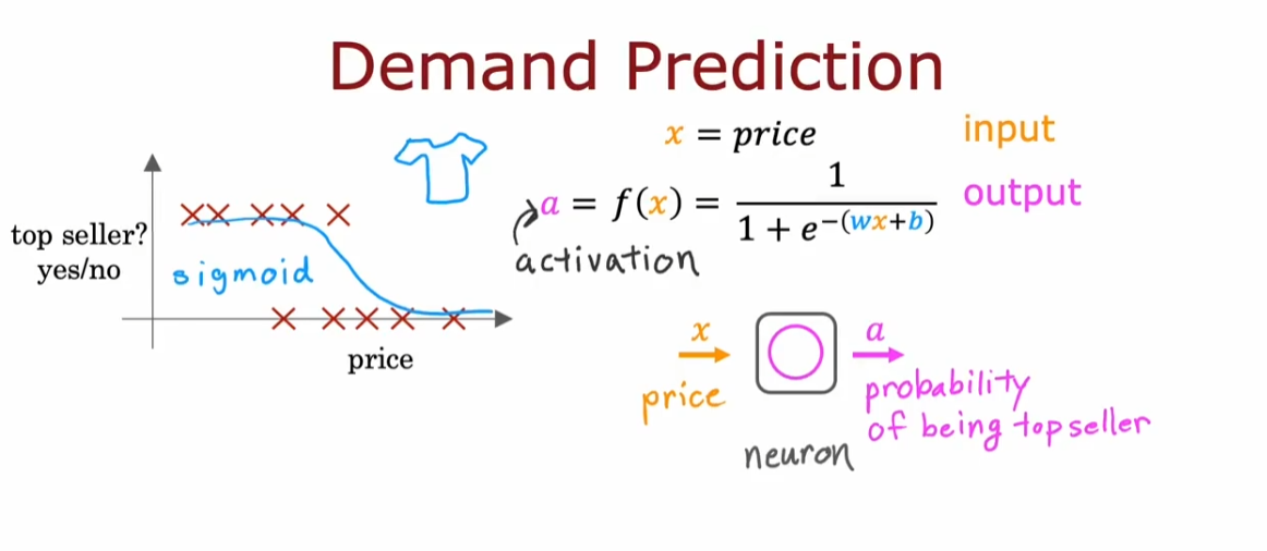
可以将神经元分为不同层（layer），每层接受相似的输入，输出不同的结果

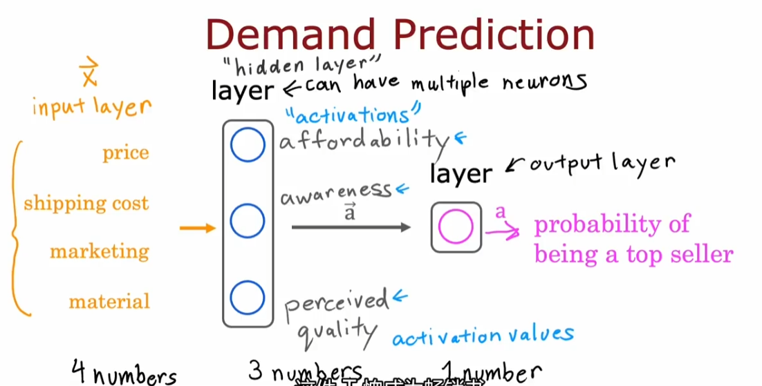
神经网络不需要自己进行特征工程，中间的隐藏层即通过输入初始特征来输出更好的特征
需要自己决定的是神经网络的架构：即有多少层，每层有多少神经元

3.1.1. 一些 notation

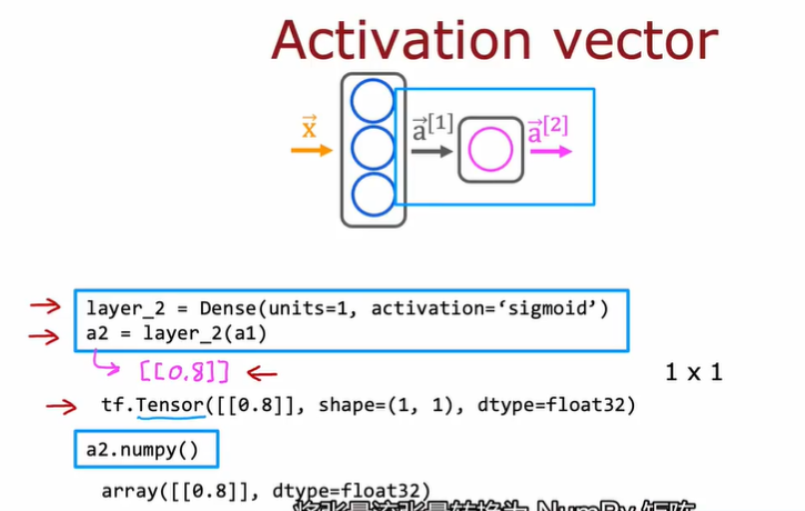
方括号上标代表第 x 层

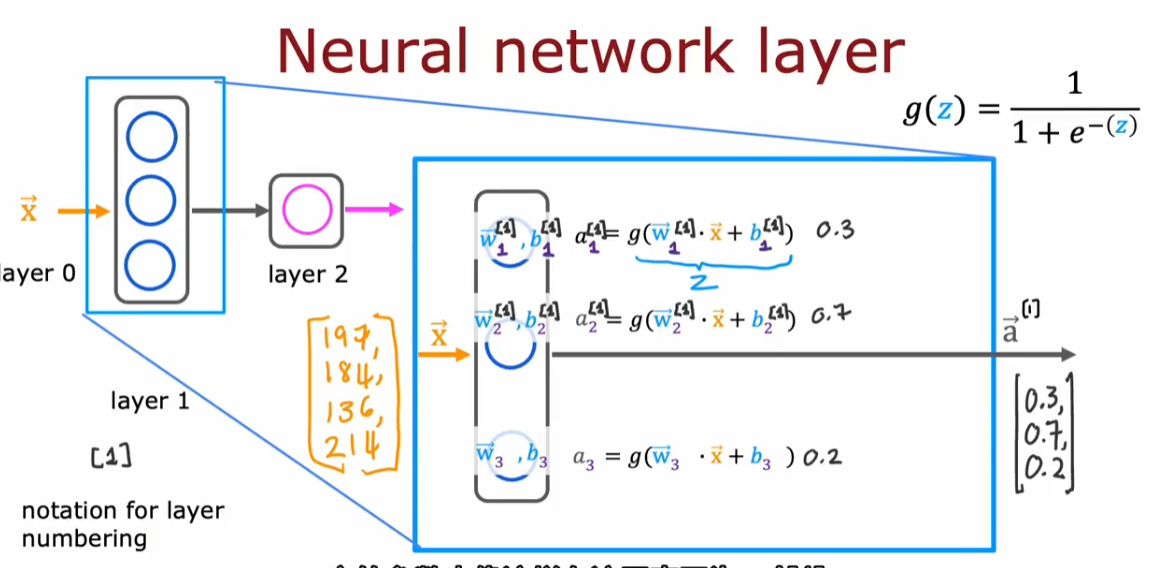
每层接受的输入向量上标是上一层的
$a^{[0]}$一般表示输入向量

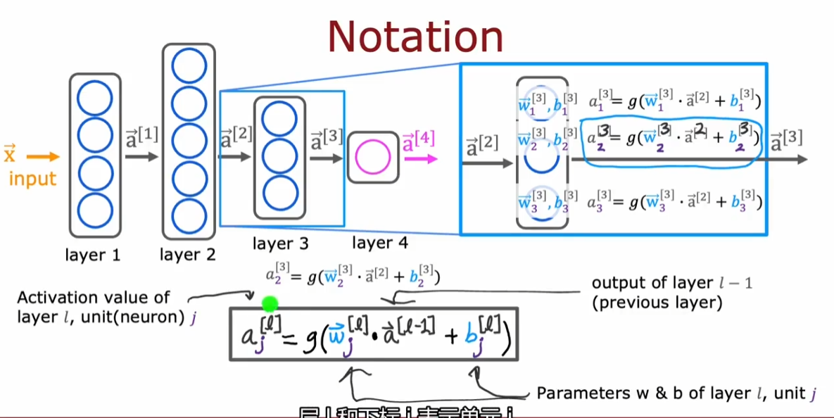
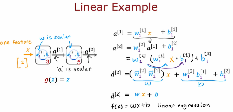
3.1.2. forward propagation

前向传播
从神经网络层自左向右传播

3.2. TensorFlow 介绍

3.2.1. Demo

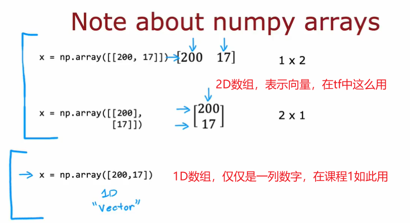
x = np.array([[200.0, 17.0]])
# Dense是神经网络一种层的名字
layer_1 = Dense(units=3, activation='sigmoid')
# a1是一个1 * 3矩阵（张量），通过a1.numpy()可以把它转换为numpy矩阵
a1 = layer_1(x)
layer_2 = Dense(units=1, activation='sigmoid')
a2 = layer_2(x)

# Threshold
if a2 >= 0.5
	yhat = 1
else:
    yhat = 0


# 法2
layer_1 = Dense(units=3, activation='sigmoid')
layer_2 = Dense(units=1, activation='sigmoid')
model = Sequential([layer_1, layer_2 ])
x = np.array([[]])
y = np.array([[]])
model.compile(...)
model.fit(x,y)
model.predict(x_new)

3.2.2. Tf 的数据格式

3.2.3. Tensor（张量）

可以近似理解为一种矩阵

3.3. Python 向前传播的原理

forward prop
手写全连接层（full connected）

def dense(a_in, W, b, g):
    units = W.shape[1]
    a_out = np.zeros(units)
    for j in range(units):
        # W[:,j]是提取出W第j列的写法
        # 通常：大写字母用来表示矩阵，小写字母用来表示向量
        w = W[:,j]
        z = np.dot(w, a_in) + b[j]
        a_out[j] = g(z)
    return a_out

def sequential(x):
    a1 = dense(x, W1, b1)
    a2 = dense(a1, W2, b2)
    a3 = dense(a2, W3, b3)
    a4 = dense(a3, W4, b4)
    f_x = a4
    return f_x

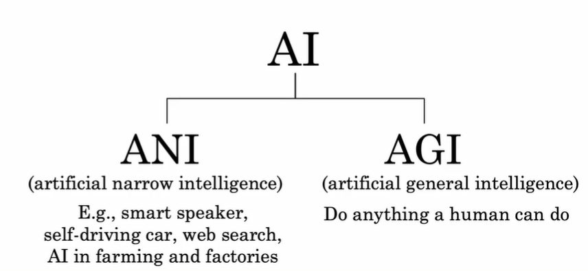
3.4. AI 和神经网络的关系

3.4.1. ANI 和 AGI

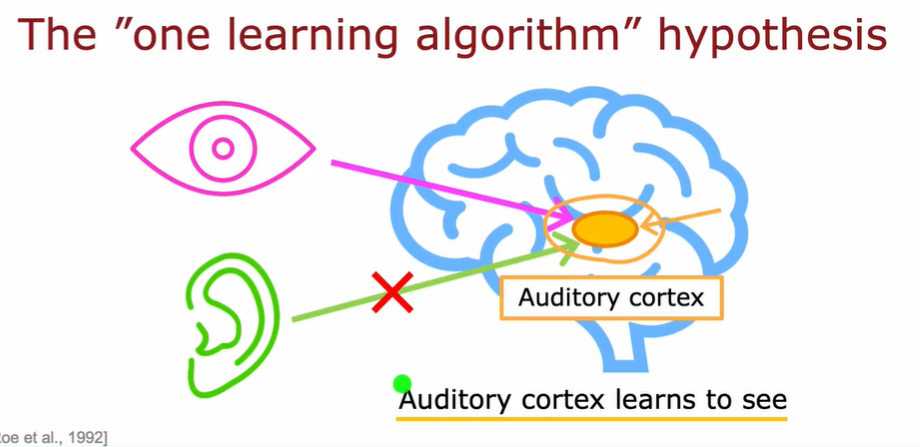
3.4.2. The “one learning algorithm” hypothesis

科学家发现人脑的可塑性非常强：非常小的一片人脑区域就能做很多事情，比如当把图像输给听觉区域时，听觉区域又会学会识别图像。这带来一个假设：存在一种或几种算法，可以使得机器学习/神经网络实现非常多的事情

3.5. 算法中的向量化实现

X = np.array([[200, 17]])
W = np.array([[1, -3, 5],
              [-2, 4, -6]])
B = np.array([[-1, 1, 2]])

def dense(A_in, W, B, g):
    # np.matmul = matrix multiplication
    Z = np.matmul(A_in, W) + B
    A_out = g(z)
    return A_out

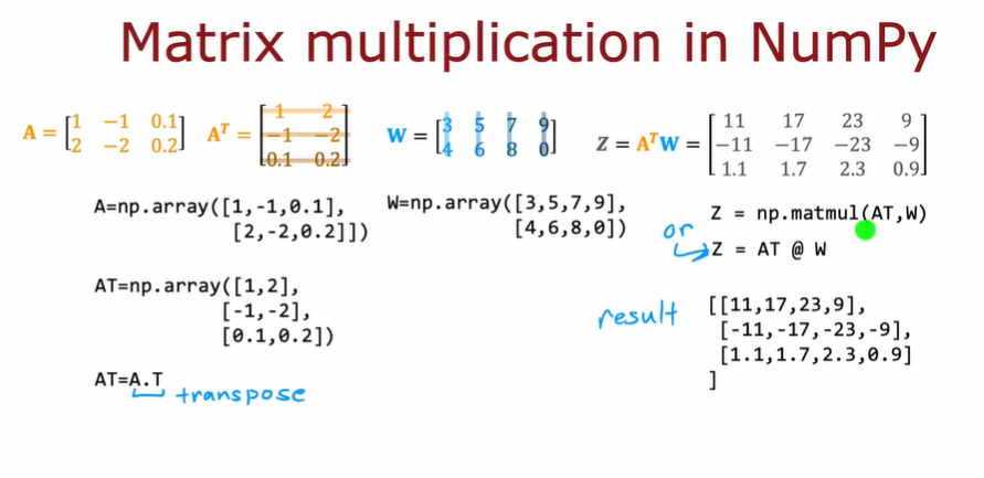
使用矩阵和向量运算的好处是：可以利用硬件进行并行计算，显著提高运算速度
在 TensorFlow 的约定中：一个样本的数据通常在矩阵的行中

3.6. TensorFlow 实现

tf 编译模型的关键是定义损失函数
第一步：定义模型
第二步：使用损失函数编译模型
第三步：训练模型

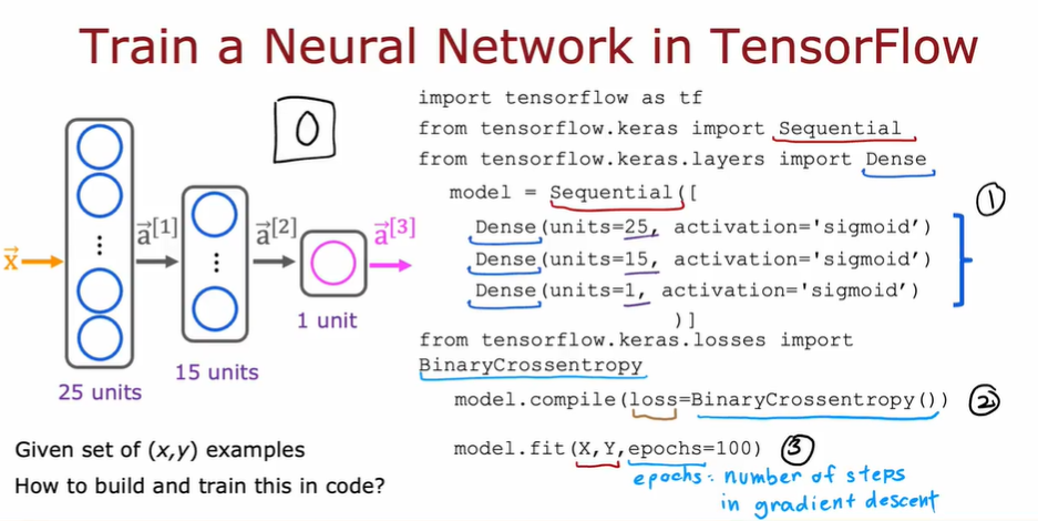
3.6.1. 前述基本步骤在 tf 中的对应

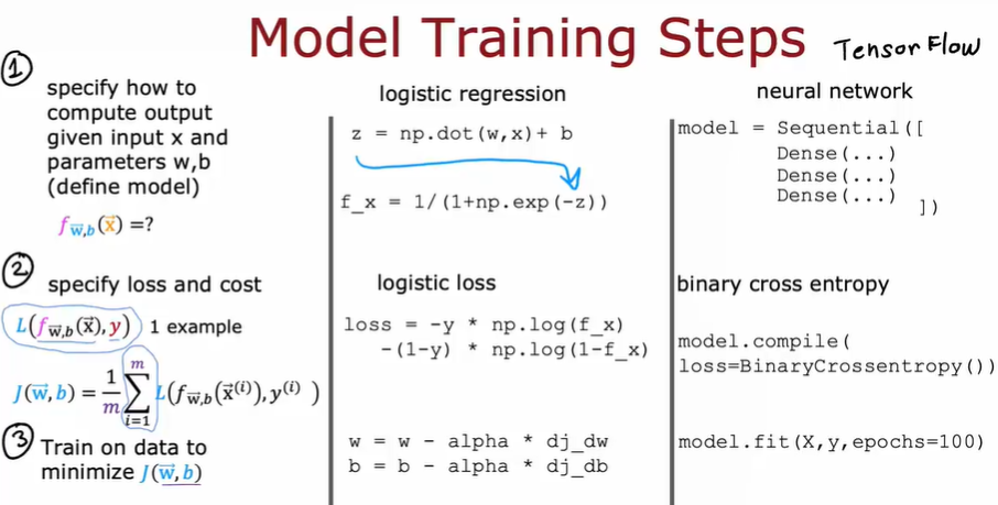
tf 的 model.fi 通过反向传播实现了梯度下降

3.7. 激活函数详解

一些激活函数

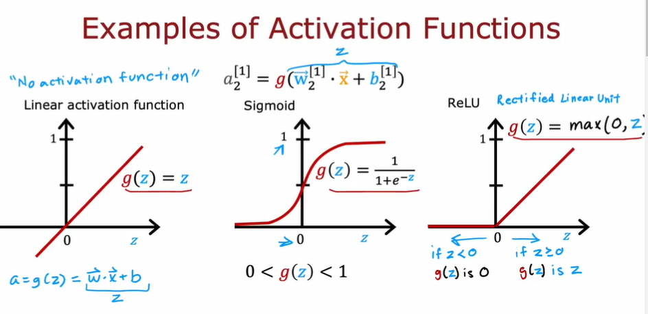
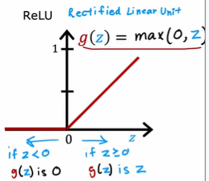
3.7.1. ReLU

Rectified Linear Unit 修正线性单元
计算速度比 sigmoid 更快
只有左端是趋于 flat 的，因此在梯度下降时比 sigmoid 更有优势，学习速度更快
一般作为隐藏层的默认激活函数

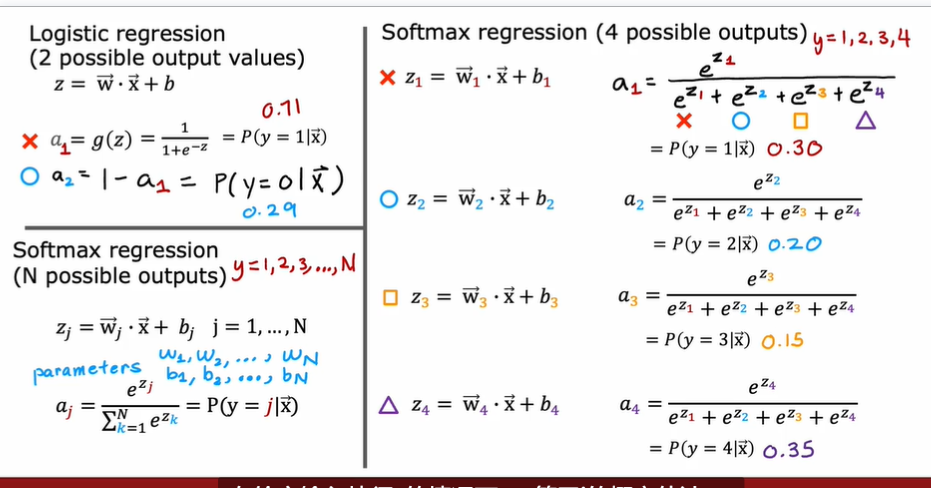
3.7.2. softmax

逻辑回归的泛化
针对多分类环境

3.7.2.1. softmax 函数的损失函数

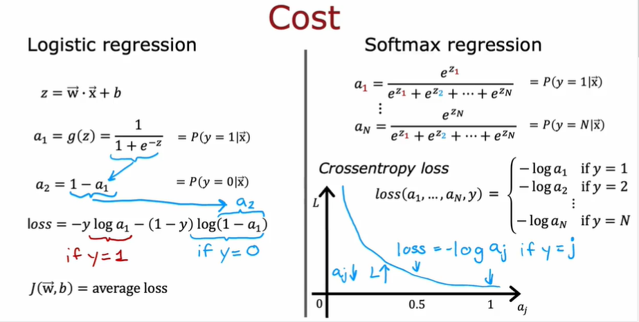
可以和 sigmoid 类比，$a_j$越接近 1，损失越小，这会刺激$a_j$不断接近 1

3.7.3. 如何选择激活函数

sigmoid：二元分类问题，因为神经网络在学习 y=1 的概率
linear：回归
ReLU：回归，且结果是非负值

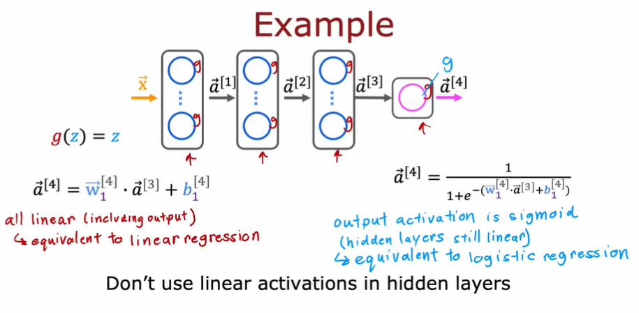
3.7.4. 为什么我们需要激活函数

简单来说，如果我们不使用激活函数，那么所有神经网络将变成如同线性回归般的简单计算。多层神经网络不能提供提升计算复杂特征的能力，也不能学习任何比线性函数更复杂的东西，违背了我们创造神经网络的初衷

3.8. 多分类

y 是离散的，且可能的取值大于 2 种
使用 softmax 激活函数

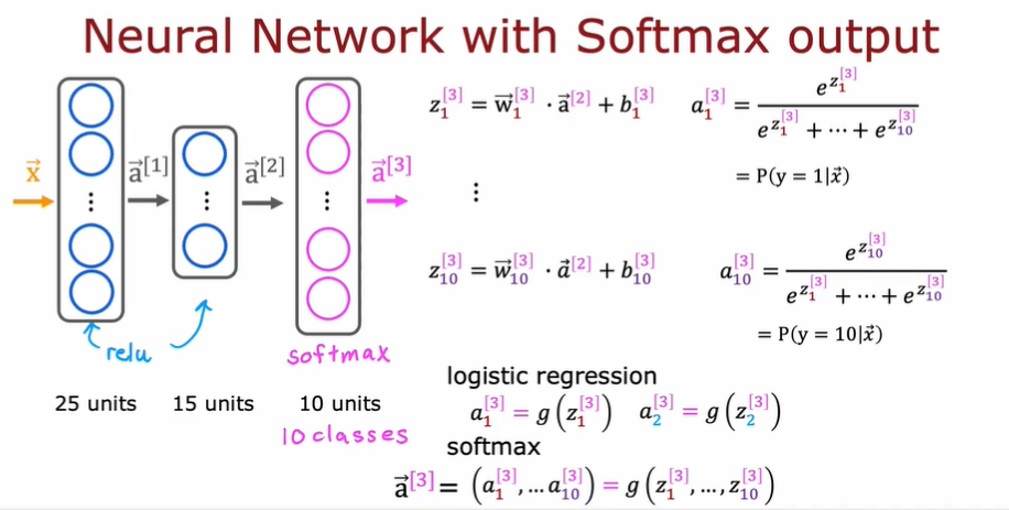
softmax 函数在这里和其他激活函数的区别是，softmax 函数一次性算出$a_1, a_2, …, a_i$的所有值，并计算出它们的概率。而其他激活函数仅仅只是一次计算出一个。

3.8.1. 使用 tf 实现

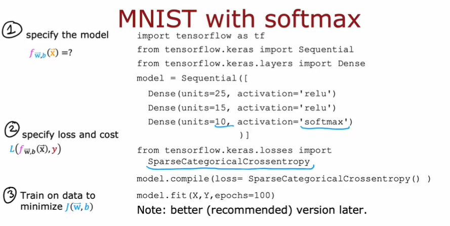
一种 tf 实现的版本，但是实际上有更好的版本。因此

3.8.1.1. 优化计算精度

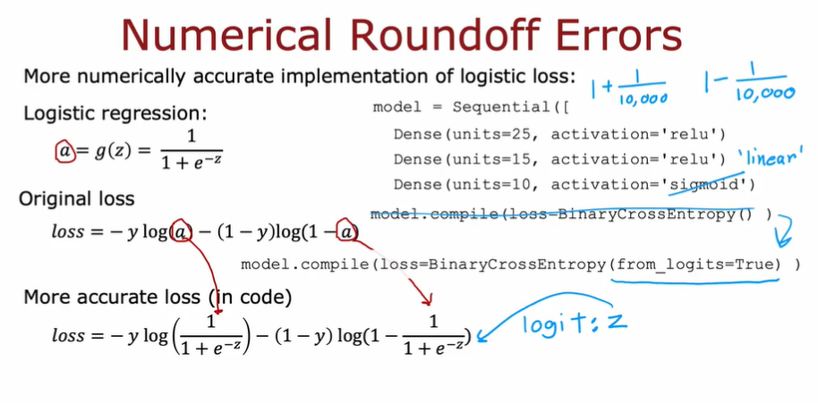
在输出层使用 linear 激活函数（目的是为了不先计算 a/z，而是把整个式子放到最后再统一计算，避免了计算中间值而带来的精度误差），然后在 compile 选项里加上from_logits=True

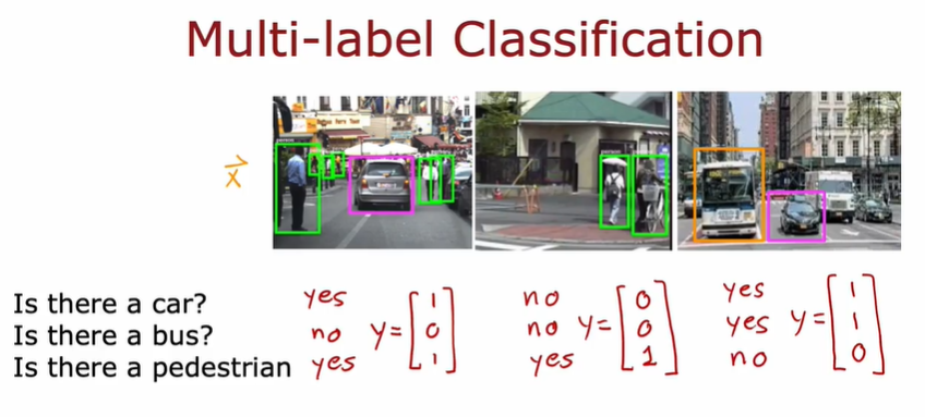
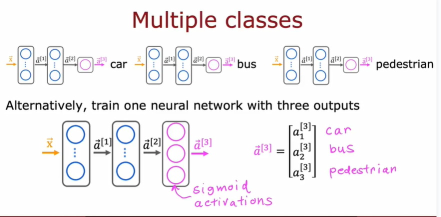
3.8.2. 多标签分类问题

multi-label classification problem
输出是一个标签向量，表示是否包含某个向量

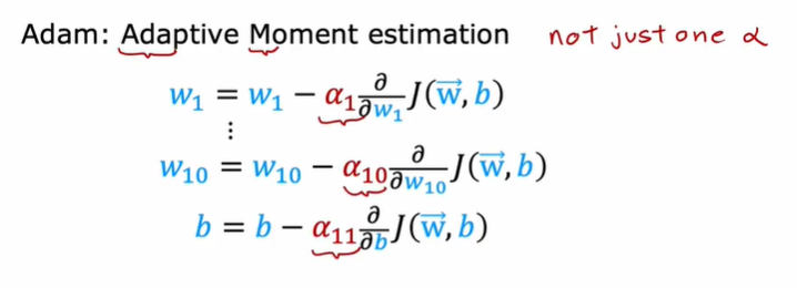
3.9. Adam 算法

Adaptive Moment estimation，自适应矩估计
可以自动调整学习率$\alpha$
对于不同模型使用不同$\alpha$

3.9.1. 使用

model = Sequential([
    Dense(units=25, activation='sigmoid')
    Dense(units=15, activation='sigmoid')
    Dense(units=10, activation='linear')
])

model.compile(optimizer=Adam(learning_rate=le-3),                loss=SparseCategoricalCrossentropy(from_logits=True))

model.fit(X,Y,epochs=100)

在 compile 里面加一个优化器参数即可，然后设置一个默认的学习率

3.10. Layer Types

3.10.1. Dense layer

全连接层，接受前一层的所有激活，然后通过一个激活函数得到它自己的输出

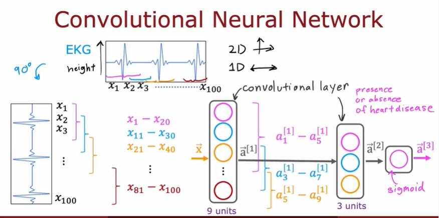
3.10.2. Convolutional Layer

卷积层

每一个神经元只关注**part of**前一层的输出
优点：
- 计算更快
- 所需的训练数据更少，也更不容易过拟合
例子
可选择参数：每层的神经元数，每个神经元得到的输入数量

May 15, 2022

Coursera: ML03-深度学习